SciPy ODR

ODR 代表 正交距离回归 ，用于回归研究。基本线性回归常用于估计两个变量之间的关系 y and x 通过在图表上绘制最佳拟合线。

用于此的数学方法被称为 最小二乘 ，并旨在最小化每个点的平方误差之和。这里的关键问题是如何计算每个点的误差(也称为残差)？

在标准线性回归中，目的是根据 X 值预测 Y 值——因此明智的做法是计算 Y 值的误差(如下图的灰线所示)。但是，有时将 X 和 Y 的误差考虑在内更为明智(如下图中的红色虚线所示)。

例如： 当你知道你对 X 的测量是不确定的，或者当你不想关注一个变量相对于另一个变量的误差时。

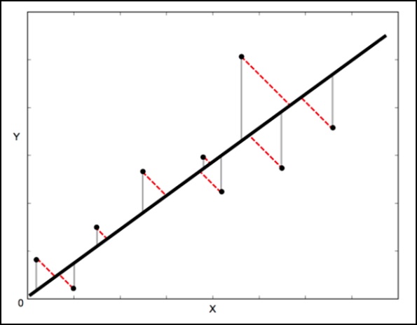
正交距离回归 (ODR) 是一种可以做到这一点的方法(在这种情况下，正交意味着垂直——因此它计算垂直于线的误差，而不仅仅是“垂直”)。

scipy.odr 单变量回归的实现

以下示例演示了单变量回归的 scipy.odr 实现。

import numpy as np
import matplotlib.pyplot as plt
from scipy.odr import *
import random

# Initiate some data, giving some randomness using random.random().
x = np.array([0, 1, 2, 3, 4, 5])
y = np.array([i**2 + random.random() for i in x])

# Define a function (quadratic in our case) to fit the data with.
def linear_func(p, x):
    m, c = p
    return m*x + c

# Create a model for fitting.
linear_model = Model(linear_func)

# Create a RealData object using our initiated data from above.
data = RealData(x, y)

# Set up ODR with the model and data.
odr = ODR(data, linear_model, beta0=[0., 1.])

# Run the regression.
out = odr.run()

# Use the in-built pprint method to give us results.
out.pprint()

上述程序将生成以下输出。

Beta: [ 5.51846098 -4.25744878]
Beta Std Error: [ 0.7786442 2.33126407]

Beta Covariance: [
    [ 1.93150969 -4.82877433]
    [ -4.82877433 17.31417201
]]

Residual Variance: 0.313892697582
Inverse Condition #: 0.146618499389
Reason(s) for Halting:
    Sum of squares convergence